A First Time Use of a CNN and a Confusion Matrix For Results
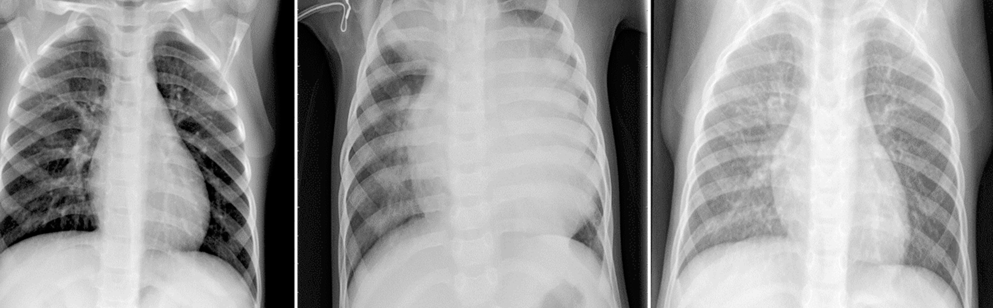
During my studies I've decided to use deep learning neural networks to build an algorithm that classifies a set X-rays images belonging to pediatric patients to help determine if whether or not pneumonia is present. The goal is to help the patient by knowing sooner than later if pneumonia is present so that treatment could begin promptly. The Neural Network I've chosen was the Convolutional Neural Network (CNN) since it is highly preferred for image processing.
What is CNN?
A Convolutional Neural Network (CNN/ConvNet) is a Deep Learning algorithm that can take in an image, assign importance (learnable weights and biases) to various aspects/objects in the image and be able to differentiate one from the other. The pre-processing required in a CNN is much lower as compared to other classification algorithms. In simpler terms, the role of the CNN is to reduce the images into a form that is easier to process, without losing features that are critical for getting a good prediction.
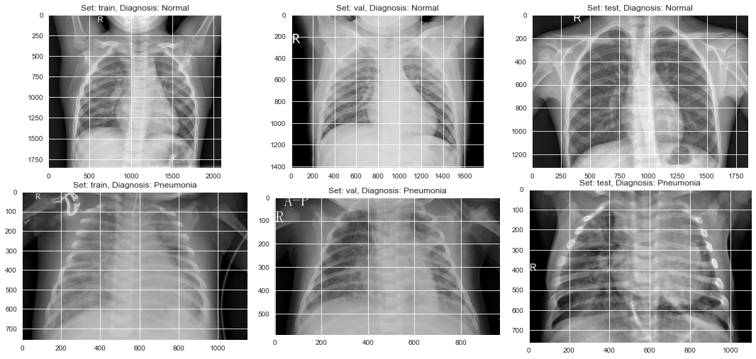
For my project I've used data sourced from kaggle.com. Upon initially exploring the data, I noticed it contained 5,756 X-ray images.
Modeling
After preprocessing the data (I've used image rescaling as well as data augmentation -- this is the process of "augmenting" the data by artificially creating new training data from the existing data by applying a number of techniques such as flipping, zooming, etc.), I've built my model by doing the following:
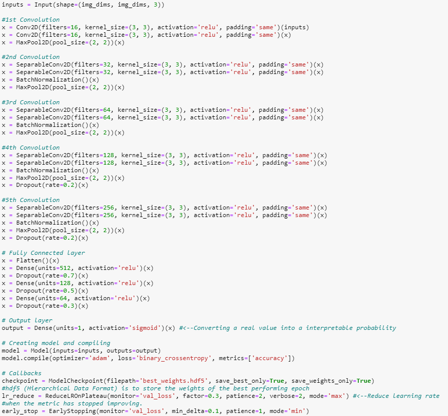
1- Using five convolutional blocks comprised of convolutional layers, BatchNormalization, and MaxPooling.
2- Reducing over-fitting by using dropouts. (4)
3- Using ReLu (rectified linear unit) activation function for all except the last layer. Since this is a binary classification problem, Sigmoid was used for the final layer. (5)
4- Using the Adam optimizer and cross-entropy for the loss. (6)
5- Adding a flattened layer followed by fully connected layers. This is the last stage in CNN where the spatial dimensions of the input are collapsed into the channel dimension.
Note:
- ReLu: a piecewise linear function that outputs zero if its input is negative, and directly outputs the input otherwise.
- Sigmoid: its gradient is defined everywhere and its output is conveniently between 0 and 1 for all x. (5)
After testing 8 models, I've chosen the following since it has offered satisfactory results based on both its validation and test accuracy. The final model is a five Convolution Block model with twin (double) Conv2D per block and Dropout of 0.2. This model follows the VGG16 format, more of which can be learned about here.
All of the 8 models were initially trained with 10 and 15 epochs and was increased to 50 when the validation accuracy increased to more than 70%. I've attempted to increase the epochs to 100 however my system couldn't handle the burden. This particular model took 10 hours to train!
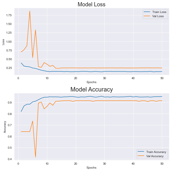
The simplest way to analyze the performance of a model is to examine a visualization of its results. So after many hours of training, my algorithm produced the following results:
 )
)
As can be seen above, the curves of the validation accuracy and the loss indicate that the model may converge with more than 50 epochs (though it hasn't happened with the ones its been fitted with). As I've previously mentioned, I've attempted to train for more epochs and larger batch sizes but have been unsuccessful.
It's clear from the train accuracy that the model is overfitted; however the model's accuracies were still decent with the test subset. The results were:
- Accuracy: 91.22137404580153%
- Precision: 90.38461538461539%
- Recall: 96.76470588235294%
- F1-score: 93.4659090909091
It's important to note in evaluating this model that accuracy is an inappropriate performance measure for imbalanced classification problems such as this. This is because the high number of samples that form the majority class (training subset) overshadows the number of examples in the minority class. This translates to accuracy scores as high as 99% for unskilled models, depending on how severe the class imbalance is.
As an alternative better option, using precision, recall and F-1 metrics can offer more reliable results. These metric concepts are are follows:
Precision: quantifies the number of correct positive predictions made: it calculates the accuracy for the minority class. = tp/(tp + tp)
Recall: quantifies the number of positive class predictions made out of all positive examples in the dataset. It provides an indication of missed positive predictions. = tp/(tp + fn)
F1-Score: balances both the concerns of precision and recall in one number. A good F1 score means low false positives and low false negatives = (tp + tp)/total
Note: tp = true positive, tn = true negative, fp = false positive, and fn = false negative [See above source for reference]
To better understand these metrics, it's often very helpful to plot a confusion matrix to accurately interpret the results. It's important to keep in mind that the most important one is Recall, because a patient would prefer that his/her doctor misdiagnosed them with pneumonia when in fact they don't, over a misdiagnosis as being healthy when in reality pneumonia is present, and in fact miss out on treatment. While Precision is an important metric, Recall for medical problems may be more accurate.
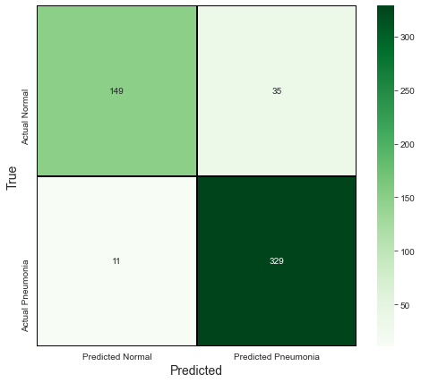
In viewing the matrix, we see 11 representing the fn and the 329 representing the tp from our model, we can deduct that this means that only 11 patients are misdiagnosed as not having pneumonia.
pool_size) for each channel of the input. The window is shifted by strides along each dimension. Soucre: MaxPooling2D layer (keras.io)rate at each step during training time, which helps prevent overfitting. Source: Dropout layer (keras.io)
Comments
Post a Comment